At the heart of the scientific process is the yearning for universal characteristics that transcend historical contingency and generalize the unique patterns observed in nature. In many cases these universal characteristics bleed across the different branches of the tree of knowledge and almost serendipitously relate disparate systems together. In the last century a growing consciousness of one such emerging universality has sparked an obsession with the ideas behind criticality and phase transitions. One domain where criticality pops up quite often is in the dynamic domain of life (and complexity), and more recently in understanding the organization of brain and society. What is becoming clear about criticality is that it isn’t just a mode of organization that is possible, it seems to be an attractor in mode-space. For whatever reason, criticality, the self-organization of criticality, and evolution are deeply intertwined and it is the goal of this project to explore this intersection of ideas.

The present post was written by Sina Khajehabdollahi, and is the product of a collaboration with Olaf Witkowski, funded partly by the ELSI Origins Network. This research will be published in the Proceedings of the 2018 Conference on Artificial Life (ALIFE 2018), which will take place in Tokyo, Japan, July 23-27, 2018.

Criticality and Phase Transitions

Modes of Matter and their Collective Organizational Structures

Our understanding of the phases of matter start from ancient beginnings and have their origins rooted in the phenomenological experience of the world rather than scientific inquiry. Earth, Water, Air, Earth, Aether, from these everything is made, or so was/is thought. We have since moved on to more ‘fundamental’ concepts like quarks and electrons, waves and plasmas; Modes of matter and the ways that they can organize.

Is this a recursive process? Is ‘matter’ simply a sufficiently self-sufficient ‘mode of organization’? The brain as a phase of neural matter? The human as a phase of multi-cell life, multi-cell life as a phase of single-cell life, single-cell life a phase of molecular matter, etc.

Matter: A self-sufficient mode of organization with ‘reasonably’ defined boundaries.

The phases of nature are most prescient when they are changing, for example observing the condensation of vapor, the freezing of water, the sublimation and melt of ice. Emphasis must be put on the notion that phase transitions are generally describing sudden changes and reorganization with respect to ‘not-so-sudden’ changes in some other variable. In other words, phase transitions tend to describe how small quantitative changes can sometimes lead to large qualitative ones.

Associated with phase transitions are critical points (or perhaps regimes in the case of biological systems), where these critical points are analogous to a goldilocks zone between two opposing ‘ways of organization’. In an abstract/general sense, a critical point is the point where order and disorder meet. However, there may certainly be times where there are transitions between more than 2 modes of order. By tuning some choice of ‘control parameter and measuring your mode of ‘order’, a phase diagram can be plotted. In the case of Figure 1, this is seen for the control parameters temperature and pressure for relatively ‘simple’ statistical physics systems.

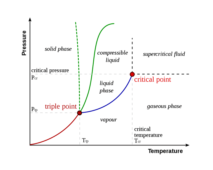
However, such a plot is not readily available when discussing complex systems like humans or human society and its idiosyncratic modes of interaction, partially for a lack of computational power which is constantly improving, but fundamentally due to our constrained knowledge of complex/chaotic systems and their descriptive mathematics.

Finally, the importance of criticality arises from this ‘best-of-both-worlds’ scenario, given that the ‘both worlds’ are distinct and useful modes of order/disorder. For example in the conversation of the human brain, the dichotomy is often between segregation and cooperation; The brain is a modularly hierarchical structure of interconnected neurons which have the ability to take advantage of ‘division-of-labor’ strategies while also being capable of integrating the divided labor into a larger whole. There seems to be an appropriate balance of these forces, between efficiency and redundancy, between determinism and randomness, between excitation and inhibition, etc. The most appropriate ‘order parameter’ is not obvious and there are many choices possible along with many more choices for ‘control parameters’.

We need a sufficiently simple model to play with, and to that end we look to the Ising model.

Ising Model

Phenomenological model of phase transitions

The Ising model is probably the simplest way to model a many-body system of interacting elements. In its simplest form (at least the simplest that exhibits phase transitions), binary elements that can only take the values of ±1 are organized onto a 2D lattice grid, interacting only with their nearest neighbours. This model can be an analogy for solid matter or gasses with local interactions as it originally inspired, but also now more generally for modelling neurons in the brain, or humans or agents in socio-economic contexts.

The success of this simple model was in its ability to exhibit a phase transition by changing only one control parameter, the temperature of the heat bath. As the temperature increased, larger and larger energetic fluctuations are allowed where the Energy of a system in a configuration is:

$$ E = – \sum_{\left \langle i, j \right \rangle} J_{i,j} s_i s_j – \sum_i h_i $$

where the summation \( \left \langle i, j \right \rangle \) is over all nearest neighbours, \( J_{i,j} \) is the interaction strength between nodes \(i\) and \(j\), and \(h_i\) is the locally applied field/bias. The model tends to try to minimize its energy by favouring the probability of ‘spin-flips’ that minimize \(E\). Unfavorable spin-flips are allowed as a function of a Boltzmann factor:

$$ p \sim e^{\frac{\Delta E}{T}} $$

As the control parameter temperature is varied, the system can act more or less randomly. A critical temperature exists such that the qualitative organization of the model becomes discontinuous and changes. At the critical point, the system exhibits long-range correlations and maximizes information transfer between nodes, properties deemed extremely useful if not necessary for intelligent systems.

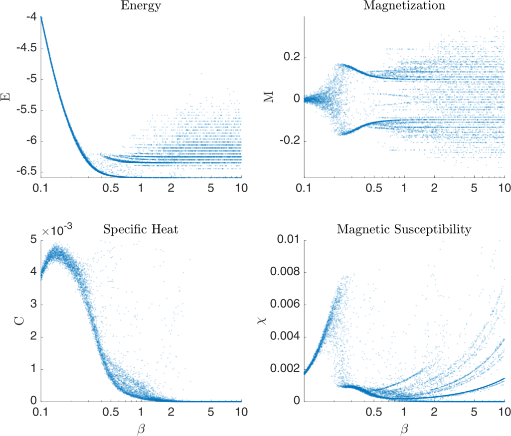
Figure 3 visualizes some basic statistical measures of an example Ising system as a function of \( \beta = 1/T \) simulated using Monte Carlo Metropolis methods. In this case instead of a 2D lattice grid, a fully-connected graph with normally distributed (mean 0) random edge weights is generated. The transition point of this model is most easily discerned in the discontinuity of the Magnetic Susceptibility plot, though the transition exhibits itself in the other variables quite noticeably as well.

Ising-embodied Neural Networks

It’s Alive! Making the Ising model do things!

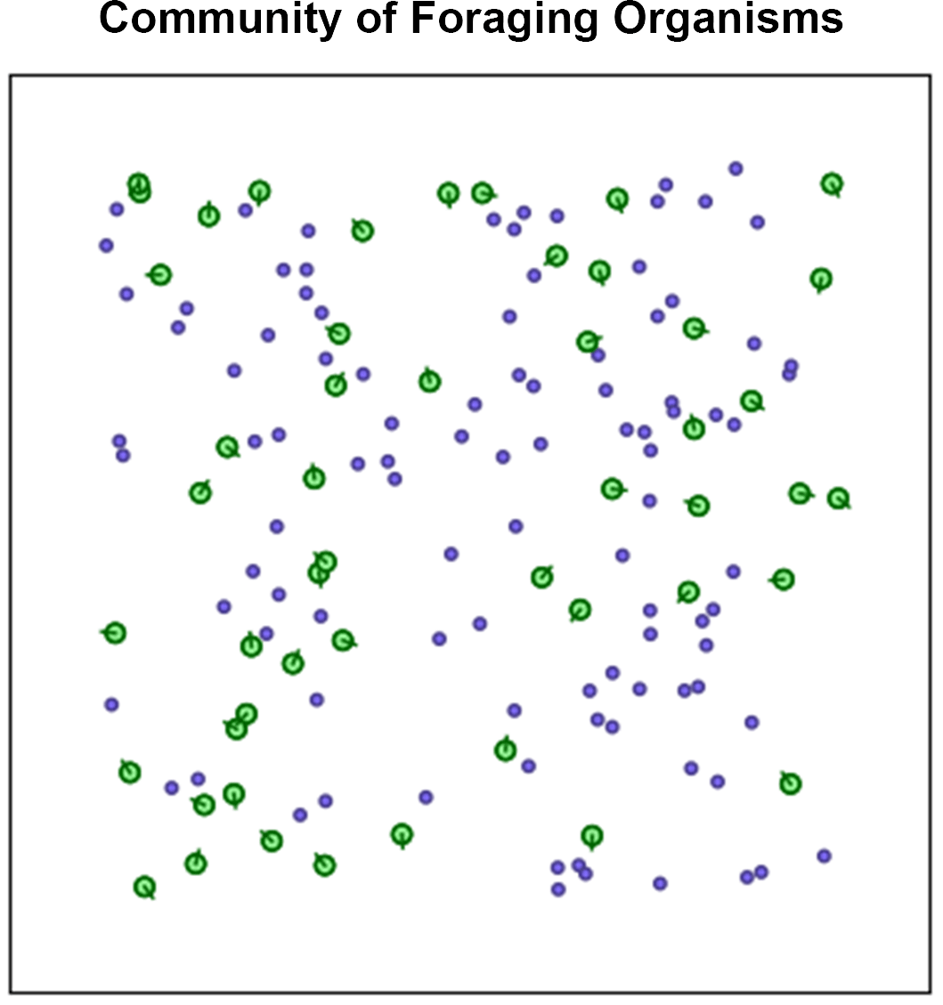
Now the point of this project wasn’t simply to play with any old Ising models, the goal was to embody these Ising models into context and bring them to life so that we can see how/if criticality may play a role in adaptation and survival. To that end, we introduce the Ising organism, an object class that has its own unique connectivity matrix and acts as an independent neural network organism as visualized in Figure 4.

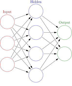
The sensor neurons for these organisms are sensitive to the angle to the closest food, the distance to the closest food, and a directional proximity sensor with respect to other organisms. These sensor (input) neurons are connected to a layer of hidden neurons, which are in turn connected to both themselves and motor (output) neurons. The motor neurons control the linear/radial acceleration/deceleration, effectively identical to the steering wheel and gas/brakes in a car.

A community of 50 organisms with this architecture (but each with its own set of unique weights) are generated and placed in a 2D environment that spawns food (Figure 5). A generation is defined as an arbitrary amount of time (for example 4000 frames) where all organisms can explore their environment by moving around. When an organism (green circles) gets close enough to a parcel of food (purple dots), the food disappears, and a counter adds to the score of the organism. Food parcels respawn instantly upon being eaten so there is always an infinite supply.

From here, we can begin to explore ways in which these Ising-embodied organisms can adapt to their environment.

Critical Learning

Strategies for approaching criticality

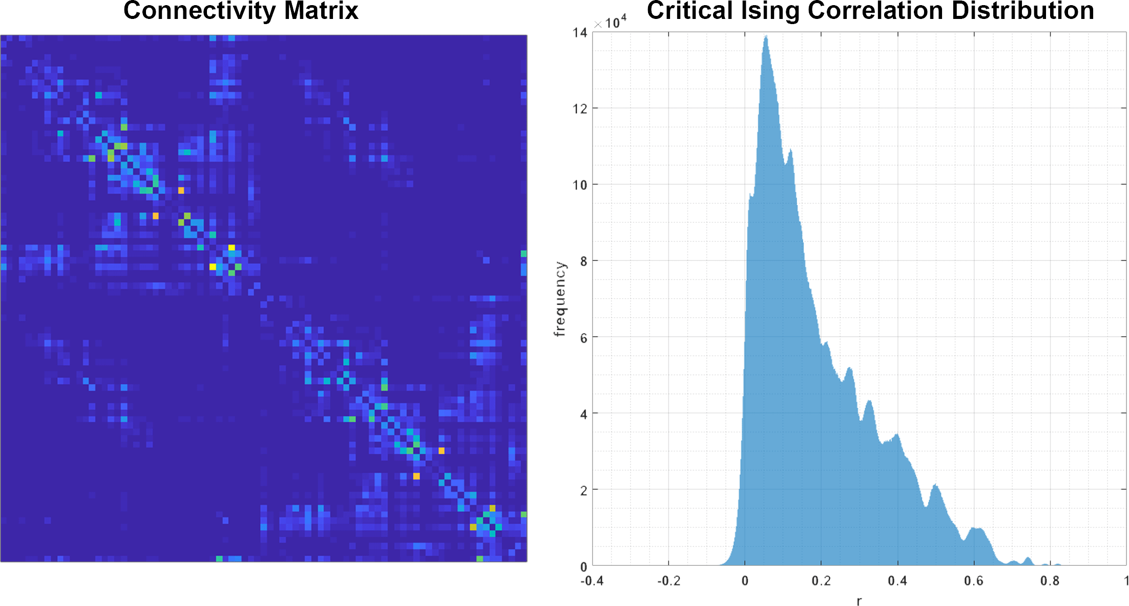
Initially this project was motivated by “Criticality as It Could Be: organizational invariance as self-organized criticality in embodied agents” a project by Miguel Aguilera and Manuel G. Bedia. In their work they demonstrate that criticality can be learned in an arbitrary Ising-embodied neural network simply by applying a gradient descent rule to the edge weights of the network. The gradient descent rule would attempt to learn a distribution of correlation values which are assigned to it a priori (Figure 6). The gradient descent rule governs the adaptation of the organism:

$$ h_i \leftarrow h_i + \mu (m_i^* – m_i^m) \\ J_{ij} \leftarrow J_{ij} + \mu (c_{ij}^* – c_{ij}^m) $$

The local fields and interaction strengths (edge weights) are updated with respect to the actual mean activation \( m_i^m  \) and the reference activations \( m_i^*  \) from the known critical system and similarly for the actual correlation values \( c_{i,j}^m  \) versus the reference correlation value \( c_{i,j}^*  \) from the known critical system.  \( \mu = 0.01 \) is the learning rate. We introduce a concept analogous to that of the generation, the semester, an arbitrary number of time points (again, 4000 frames for example) in which the organisms have time to generate correlation/mean activation statistics at the end of which the gradient descent rule is applied. In short, the gradient descent rule is applied once per semester.

By learning the correlation distributions of a known critical, Ising system, an arbitrary network could also learn to be critical without fine-tuning any control parameter like temperature.

Aguilera et al. embody these networks in simple games (car in a valley, double pendulum balancing) and demonstrate that once the systems converge towards criticality that the agents maximized their exploration of phase space and would position themselves at the precipice of behavioural modes. However, what success these agents demonstrated in critical learning, exploration and playfulness, they lacked in their ability to actually play these games to win. Arguably, these goals may ultimately be perpendicular, however in trying to contextualize criticality with life-like systems we must push forward and see if we can apply critical learning and evolutionary selection simultaneously.

Genetic Algorithm and Evolutionary Selection

Playing games, competing for high scores, mating, mutating and duplicating

Parallel to the critical learning algorithm, we introduce a genetic algorithm whose goals are simply to reward those organisms that have eaten the most food. Using a combination of elitist selection and mating, successful organisms are rewarded by duplication and the chance to mate and generate offspring. Mutations accompany this process and allow for the stochastic exploration of the organisms’ genotype space.

Using the previously defined concept of a generation, the genetic algorithm is applied once at the end of each generation.

Visualizing Community Evolution

Observing the evolution/learning process

So we now have a community of Ising-embodied organisms playing a foraging game in a simple, shared, 2D environment in which we introduce the concept of generations (time span in which genetic algorithm operates) and semesters (time span in which critical learning algorithm operates).

Let’s look at these 2 algorithms once each separately, and then once again together. However, when combining the two algorithms, we face a dilemma. These two adaptation algorithms tend to destroy the learning done by the other. In other words, the genetic algorithm does not conserve what is learned by the critical algorithm and vice versa. However, perhaps if we combine these two algorithms in some appropriate ratio of time scales we can achieve an adaptation scheme that is relatively continuous and non-destructive to its previous adaptations. The choice for a ratio of 6 semesters to 1 generation is made such that the learning algorithm has time to kick in before the GA can select successful foragers.

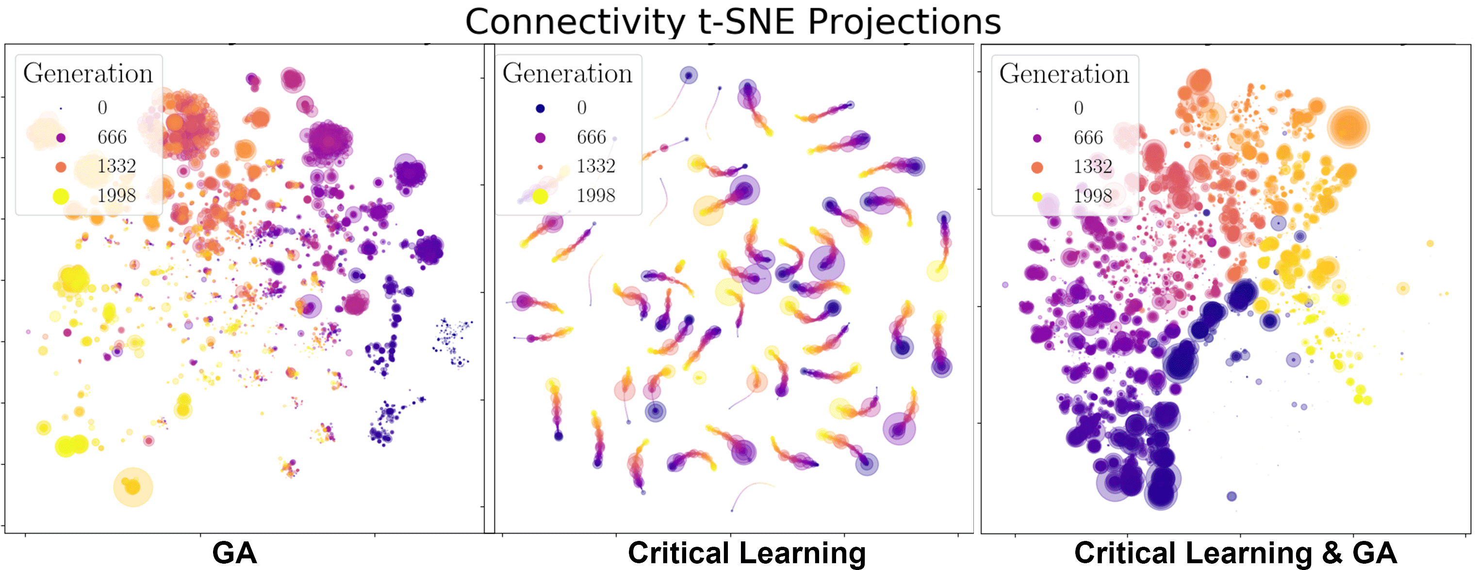
First, let’s look at how the genotypes evolve across the generations. We use tSNE projections in Figure 7 to visualize the relationships between the connectivity matrices of the different organisms. As a general clustering algorithm, tSNE projections help us visualize the groupings of high dimensional data, in this case all the edge weights in each individual neural network. We then cluster these networks across all generations to observe how they adapt either through the GA, critical learning, or both methods combined.

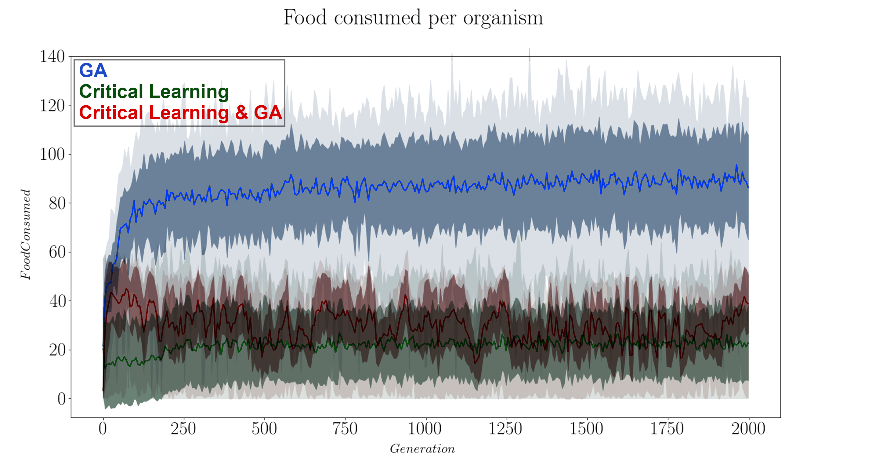
It’s useful to know how the fitness of these organisms goes across the generations, so we plot that in Figure 8 to get a feel of how well each algorithm did in playing our game.

Finally, to compare our simulations to critical systems we measure the specific heat of each organism as a function of β. If the evolution algorithm works as intended then we should see the peaks of the specific heat converge to β = 1, the β which the simulation is natively run at.

 

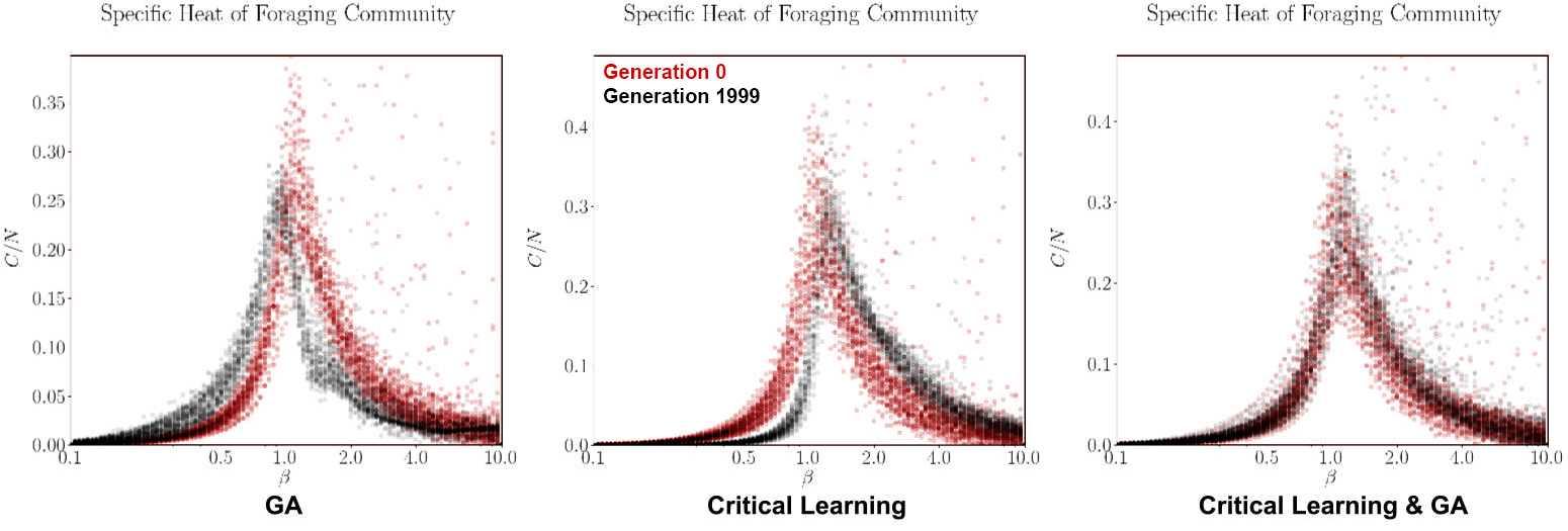
From the fitness functions in Figure 8 it is clear the GA algorithm by itself is the most successful in increasing the fitness of the organisms. This is not altogether surprising as we expected that the two algorithms will undo each other’s work if they are not appropriately made compatible. When looking at the tSNE projections of the GA algorithm by themselves we note its evolution is marked by major individual milestones (where the large clusters are) and that these organisms duplicate and seed the next generation of mutated/successful organisms. However, even this strategy plateaus quite rapidly, within approximately 250 generations. The specific heat of this paradigm both starts, and ends centered near β = 1 so it is not clear if the slight shift in the curves is within error bounds or a real pattern. We would have to run many iterations of this experiment to know for sure. Another helpful experiment that starts the community of organisms farther away from criticality (for example if we change the local temperatures (Betas) of each organism), then we might be able to better see if evolution within this foraging game drives the system towards criticality.

For the critical learning only paradigm, the tSNE projections are straight forward. Here the learning is not contingent on the fitness of the organisms at all and therefore all learning is done ‘locally’. No organisms die (because of the lack of a GA) and so there is continuity in the genotypes. This paradigm seems to act to sharpen the specific heat plots near β = 1, making for a more dramatic/steeper transition. This contrasts with the evolution algorithm which did the opposite. The fitness function of this paradigm is quite awful, again as expected since this algorithm is not learning how to play the foraging game, it is only intended to learn ‘criticality’.

Finally, when combining the two paradigms together (in a ratio of 6 semesters per 1 generation), a slightly more complicated relationship forms. In the tSNE projections we observe stronger continuity between the generations. Perhaps the critical learning algorithm here is pushing all organisms in a universal direction which clusters their genotypes closer together than the evolution only paradigm. Unfortunately however, this patter does not result in any interesting increase in the fitness function of the community, instead behaving erratically or stochastically when compared to the other two paradigms. In a sense it gives hope with respect to the critical learning only paradigm since the erratic behaviour pushes its fitness higher rather than lower. Finally, no deep insight is visible in the specific heat plots of this paradigm either as our initial condition and generation 2000 results overlap showing no indication for a trend away criticality. The failure of this experiment was to ensure that the system does not start critical!

It seems our fears have come true in a sense, the two algorithms run perpendicular to each other, each undoing the work of the last. Furthermore, our experiments had the unfortunate feature that their initial conditions were very close to criticality to begin with. This property made it difficult for us to make obvious observations. However our preliminary results seem to indicate that the evolution algorithm and the critical learning algorithm work in opposing directions. The GA tends to pull the system towards sub criticality whereas the critical learning algorithm pulled the system to super criticality (by pushing the peaks of the specific heat curves either left or right in Figure 9). There needs to be a way for both of these forces to contribute to the connectivity of the network without undoing each other’s previous learnings.

Summary

TL;DR

This project aimed to incorporate the ideas of criticality into biological, evolutionary simulations of Ising-embodied neural networks playing a foraging game. We ran 3 experiments testing 2 different adaptation algorithms (critical learning and the GA) as well as their combination is a ratio of 6 learning semesters to 1 GA generation. Our experiments results highlighted some of the short comings of our experimental set up, namely that our initial conditions were too close to criticality to begin with to distinguish any flows in parameter space. In the next experiment, communities will spawn with varying distributions of local temperatures which will force the specific heat peaks away from β = 1. This way as the community evolves, it will be much more clear if there is a flow towards β = 1 or not. Such a flow could indicate the utility of criticality. Nonetheless, in this process a set of tools were constructed for future experiments to explore further the interaction and self-organization of communities into criticality contextualized within a GA paradigm.

Finally, it was observed that critical learning and GA tend to work in opposite directions, which can be a good thing as sometimes half the battle is finding the right forms of ‘order’ and ‘disorder’. However, we were not able to reconcile these differences and instead the two algorithms tended to deconstruct each other at every turn. Future experiments in this paradigm can introduce two layers of connectivity, one for the GA and another for learning which overlap but evolve semi-independently. This reconciliation may allow for a more stable form of interaction and allow for a more diverse set of behaviours and genotypes. The idea here is that through the playful/exploratory nature of criticality, plateaus in the evolutionary process can be overcome faster thereby decreasing the time per generation to improve the community’s fitness.